A retrospective on forecasting monthly liquor demand for 8 categories across Iowa’s top 25 wholesale accounts — bigquery-public-data.iowa_liquor_sales.sales, no synthetic rows, no fabricated features. This page covers what got built, how every model was scored, the validation techniques that kept the scoring honest, and what actually held up.
A production tiered-stack pipeline forecasts weekly demand per store; a second exploration track rebuilds the problem at monthly, category-level granularity to run a much heavier model bake-off. Both are graded the same way: rolling-origin backtests against real holdout months, never a single lucky train/test split.
On the production pipeline’s weekly folds, Holt-Winters averaged 0.47 WAPE against naive’s 0.59 — a clear win for the statistical tier. Aggregate to monthly, per-category totals, and that edge disappears. Granularity changed which baseline was worth beating — see Model Comparison below.
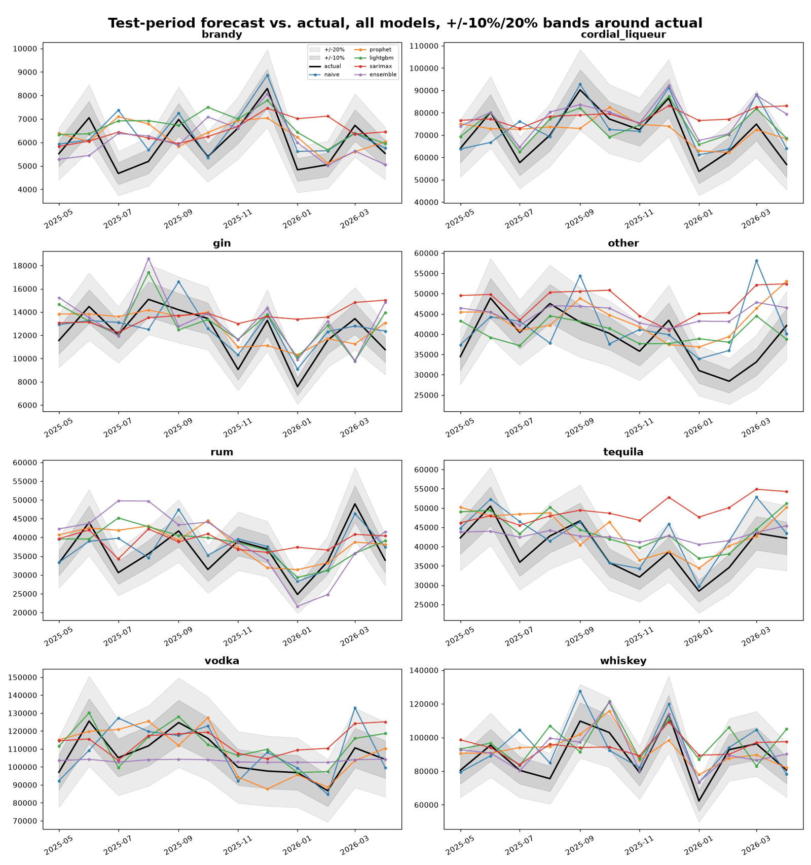
Every model was fit on training data only, forecast forward with genuine recursive rollout (never fed real future values), and scored on a 12-month holdout no model had seen. WAPE — weighted absolute percentage error — is the primary metric: lower is better. Bars below show each category’s naive baseline against its lowest-WAPE model.
Where only one bar shows, naive is the champion — a more complex model was tried and lost. other and vodka are the exceptions: LightGBM’s lag and rolling-window features found real signal a fixed year-ago lookup can’t.
| Category | Naive | Prophet | LightGBM | SARIMAX | Ensemble |
|---|---|---|---|---|---|
| brandy | 0.108 | 0.177 | 0.162 | 0.172 | 0.145 |
| cordial liqueur | 0.088 | 0.116 | 0.088 | 0.154 | 0.122 |
| gin | 0.107 | 0.122 | 0.152 | 0.159 | 0.173 |
| other | 0.172 | 0.179 | 0.141 | 0.238 | 0.177 |
| rum | 0.088 | 0.164 | 0.158 | 0.149 | 0.214 |
| tequila | 0.094 | 0.149 | 0.137 | 0.262 | 0.132 |
| vodka | 0.090 | 0.086 | 0.067 | 0.102 | 0.083 |
| whiskey | 0.094 | 0.112 | 0.161 | 0.121 | 0.134 |
Table 1 — full 12-month test WAPE, all 5 models. Highlighted cell = lowest WAPE for that row. Cordial liqueur’s tie (naive and LightGBM both at 0.088) is broken in naive’s favor — the simpler model, all else equal.
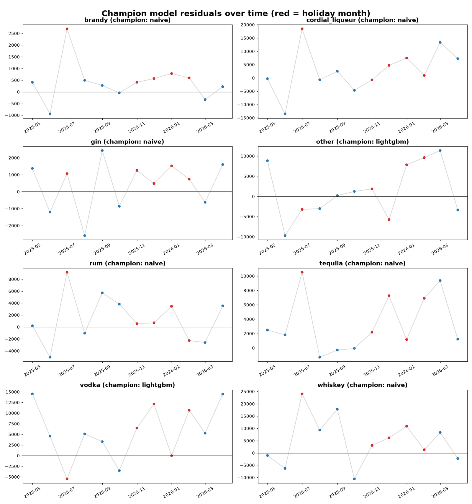
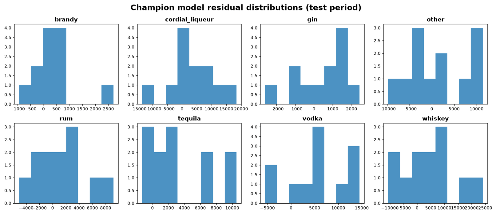
The WAPE table above is a summary; these are the actual forecasts against actual outcomes on the 12-month holdout no model — including the champion — ever trained on. All three figures are drawn from the same test-holdout run as Table 1, across all 8 categories and all 5 models.
A model that beats naive on one lucky split isn’t demonstrating skill — it’s demonstrating variance. Every technique below exists to make that distinction, and each one changed a real number when it was checked properly.
The production pipeline walks the origin forward across 6 folds, scoring point accuracy, interval coverage, and — separately — folds whose horizon overlaps the 2020 COVID window.
Exploration track: fit on train only, tune on a 6-month validation window, then refit on train+val and score once on a genuinely unseen 12-month holdout — never touched during tuning.
No distributional assumptions — just calibrated residual quantiles. But the guarantee has a real sample-size floor: 1/(1−confidence) calibration points, minimum.
The Ridge ensemble’s weights were numerically meaningless at first — alpha=3,000 behaved identically to alpha=0.1, because the penalty was invisible against a 10⁸–10₁⁰-scale loss. Standardizing first made regularization actually bite.
Stationarity was mixed, not uniform — vodka and rum tested stationary outright; brandy, cordial liqueur, and tequila didn’t. Champion-residual normality held for 7 of 8 categories.
A plain significance test found every category pair “significantly” correlated — useless. Switching to STL-residual co-movement plus an elbow cut in the linkage distances (not a hand-picked threshold) found the real structure.
At monthly, category-level aggregation with ~7 years of history, four more sophisticated models and an ensemble of all three lost to same-month-last-year on 6 of 8 categories. That’s the headline finding, and it’s reported as-is rather than buried under whichever model looks most sophisticated.
The same naive family loses more often in the production pipeline’s weekly, per-store backtests, where Holt-Winters’ extra structure has more series and more history per series to actually pay off. Aggregation level isn’t a neutral choice — it changes the honest answer.
other and vodka both improved on naive by a real, double-digit margin under LightGBM — not a rounding-error win. That’s the honest bar for “worth deploying something more complex than a lookup table.”
Price, promotions, temperature, payday timing, unemployment, consumer confidence, and CPI all appear in the original spec and none exist in this dataset. Every one is marked not available in the EDA summary rather than approximated or invented. sale_dollars is flagged as a real, unused signal for future work.
datetime64 at write time instead of requiring every downstream reader to import the exact library that could decode it.≥0 constraint was silently discarding real observations.The point of validating a forecast isn’t to make the fanciest model win — it’s to find out whether it does, and say so either way.